Collisions, Combinatorics, and Markov Analysis: `The Balance` Game Design
The Balance is a cooperative card game published by New Venture Games. The objective of the game is to set the top card on eight piles to the same value before the players run out of cards. Players do not know the contents of the other player’s hands and are restricted from communicating on the goal, so part of the challenge of the game is intuiting a shared goal. The game mechanics intersect with variants of the Birthday Paradox and similar probabilistic collision problems. We use probability, combinatorics, Markov analysis, and Monte Carlo simulation to explore the game’s design. We find that there is a sharp difficulty curve in the end game and a transition from players having many opportuntities for exploration to choosing the least-bad option that will not prevent victory.
Rules Overview
In game theory terms, The Balance is an imperfect information, stochastic, sequential, cooperative (non-zero sum), discrete game.
New Venture Games has released a video (for the general audience) explaining the rules and providing an example of play:
We have not found a link to the printed ruleset, but for our purposes we have written a formal description of the rules:
Components
- All cards have an integral value between 1 and 9, inclusive.
- The deck consists of 90 cards, ten of each value.
- The tableau consists of:
- Eight piles which accumulate face-up cards. Each pile has unlimited capacity. The top card on each pile is the value for that pile.
- The deck consists of cards that have not been drawn, nor placed in a pile, nor discarded. The deck is face-down.
- A discard area which accumulates face-up cards. This area has unlimited capacity. Players have full information on what cards have been discarded—they can search the deck at any time.
- Each player (rules suggest between 2 and 4 players) has a hand of cards with a capacity of five. The contents of each hand is private information to their player.
Initial Game State
- Deck is shuffled.
- Each player draws five cards from the shuffled deck into their hand.
- Piles in the tableau have unique initial values of 1 to 8, inclusive. These initial values do not consume cards from the deck.
Objective
All players win iff the values of all eight piles are equal at the beginning of a player’s turn. The game ends in a loss if a player is unable to perform an action on their turn due to lack of cards in their hand. A pile’s initial state (i.e. no cards placed) may contribute to a victory.
It is possible to determine the game is unwinnable without exhausting player’s hands, but we’ll usually ignore that “short circuit” option. Furthermore, the rulebook includes some game variants, which we are also ignoring in this analysis.
Gameplay
Each player takes turns in sequence and repeats until the game is completed.
On a player’s turn:
- If all eight piles show the same value: Game End - Win.
- If the player has fewer than 2 cards in their hand: Game End - Loss.
- The player performs one of four options using cards from their hand:
- Place two cards onto a target pile with the same value as the two card’s summed value modulus 10. The player chooses the order the cards are played (and thus which of the two cards becomes the pile’s new value).
- Place two cards onto one or two target piles such that each card’s values matches the target pile’s value. Both cards may be placed on the same pile if both cards share the same value. This move consumes cards from the hand but does not alter pile values.
- Place one card onto a target pile with an equal value and discard one other card. This move consumes cards from the hand but does not alter pile values. The discarded card is placed in the discard area. Then, draw a number of cards (as possible) from the deck equal to the discarded card’s value and place them in the discard area.
- Discard two cards. Place both cards in the discard area AND move cards from the deck, up to the sum of the two card’s values, into the discard area.
- Player refills hand from deck (up to two cards).
Note that exhausting the deck does not end the game. Discarded cards are not reshuffled into the deck when the deck is exhausted.
The rulebook contains additional rules on inter-player communication which we are not including in this summary.
Analysis
Are any pile values more likely than others?
No, at least not a priori. Of the 81 possible pairs of cards, there are eight pairs each that sum to each of the values between 1 and 9. There are nine pairs that sum to zero (10).
Are any pairs more useful than others?
No, at least not a priori (again). For each of the nine pile values, each has eight pairs which sum to that value modulus 10. Of the values that make up of each pair, each has equal probabilty of appearing except for the value itself, which does not appear.
For example, if a pile has a value of 3, the pair of cards that may replace it are (1, 2), (2, 1), (4, 9), (5, 8), (6, 7), (7, 6), (8, 5), and (9, 4). Each card appears twice except for 3, which does not appear in any of the pairs. This can be seen algebraically: if \(x\) and \(y\) are the two cards, \(x + y\) is the sum, but since \(x + y = x\) requires \(y\) to be zero (or ten), a pile cannot be replaced by itself under rule 3.1.
How often can players change a pile? Choose to keep the piles the same?
This is a game about collisions. Players are either altering a pile by finding a pair of cards that sums to the value (a type of collision) or trying to avoid altering pile values by finding matches (or collisions) between their cards and the piles. The difficulty is that piles must be altered before cards run out and the deck is limited.
When we think about collisions, the Birthday Paradox (aka Birthday Problem) is a good place to start (Counting Caterpillars is a good introduction). While the Birthday Paradox is about collisions within a single group, The Balance is about seeking collisions between two groups, the five cards in the player’s hand (which change over time) and the eight pile values (which have initial values but are replaced by face-up cards). Both groups are drawn from the same “bag” of cards. Cards are differentiated only by their printed value, from 1 to 9 inclusive.
If we assume mathematical independence of card draws, (Wendl 2003) has derived an exact solution to the probability of zero collisions between two sets (and thus also one or more collisions). In the paper (which is unfortunately paywalled, but Spam calls and number blocking covers the same subject by the same author), the following equation computes the probability of zero collisions between two sets of random variables, of size m and n, which contain elements that can be of any of t discrete values. For our problem, the hand size is 5, the number of piles is (up to) 8, and cards may be of 9 discrete values.
$$ P_0(m, n, t) = \frac{1}{t^{m+n}}\sum_{i=1}^{m}\sum_{j=1}^{n}S_2(m, i)S_2(n, j)\prod_{k=0}^{i+j-1}t-k $$
The function \(S_2\) computes Stirling numbers of the second kind.
This equation gives the probability of zero collisions as 1.6% or a 98.4% probability of one or more cards in the hand matching values among the piles. (Note that the hand and piles are actually bags or multisets, since they can contain duplicates, rather than sets.)
However, there are only 90 cards total in the deck. Under the assumptions of independence, the history of drawn cards should not matter. But because there are so few cards, many configurations, such as the hand and piles both being filled with 1s, are impossible (only 10 of each number is available). Hence, let’s use a Monte Carlo simulation to derive the answers numerically without assuming independence.
import collections
import itertools
from multiprocessing import Pool
import random
from dataclasses import dataclass, field
import typing

CARD = typing.Literal[1, 2, 3, 4, 5, 6, 7, 8, 9]


@dataclass
class HandCount:
    # number of hand values that are found in the pile
    value_eq: int
    # number of pairs whose sum is found in the pile
    sum_eq: int
    # number of cards that must be discarded [0, 1, 2]
    discards: int
    # minimal value of cards discarded [0, 18]
    discard_value: int


@dataclass
class PlyCounts:
    # number of simulation runs
    n_runs: int
    # number of pairs that found matches within a run
    n_pairs_match: collections.Counter[int] = field(default_factory=collections.Counter)
    # number of individual cards that found matches within a run
    n_values_match: collections.Counter[int] = field(default_factory=collections.Counter)
    # number of discarded cards
    n_discards: collections.Counter[int] = field(default_factory=collections.Counter)
    # value of discarded cards
    n_discard_values: collections.Counter[int] = field(default_factory=collections.Counter)

    def __add__(self, other: 'PlyCounts') -> 'PlyCounts':
        return PlyCounts(self.n_runs + other.n_runs,
                         self.n_pairs_match + other.n_pairs_match,
                         self.n_values_match + other.n_values_match,
                         self.n_discards + other.n_discards,
                         self.n_discard_values + other.n_discard_values)


def count_hand(hand: list[CARD], piles: list[CARD]) -> HandCount:
    count = HandCount(0, 0, 0, 0)

    for card in hand:
        if card in piles:
            count.value_eq += 1

    for pair in itertools.combinations(hand, 2):
        s = sum(pair) % 10
        if s in piles:
            count.sum_eq += 1

    if count.sum_eq == 0 and count.value_eq < 2:
        count.discards = 2 - count.value_eq
        count.discard_value = sum(sorted(hand)[:count.discards])

    return count


def montecarlo(n_runs: int) -> PlyCounts:
    counts = PlyCounts(n_runs)
    deck: list[CARD] = [1, 2, 3, 4, 5, 6, 7, 8, 9] * 10

    for _ in range(n_runs):
        random.shuffle(deck)
        hand = deck[:5]
        piles = deck[5:13]
        ch = count_hand(hand, piles)

        counts.n_pairs_match[ch.sum_eq] += 1
        counts.n_values_match[ch.value_eq] += 1
        counts.n_discards[ch.discards] += 1
        counts.n_discard_values[ch.discard_value] += 1

    return counts


if __name__ == "__main__":
    with Pool(processes=None) as pool:
        rs: list[PlyCounts] = pool.map(montecarlo, [100_000] * 100, chunksize=1)
        r = sum(rs, start=PlyCounts(0))

    # ... print statements elided ...
After 10 million runs, the results are:
        Rule 3.1
                38695 hands have 0 summing pairs (0.39%)
                97460 hands have 1 summing pairs (0.97%)
                216863 hands have 2 summing pairs (2.17%)
                725398 hands have 3 summing pairs (7.25%)
                1473089 hands have 4 summing pairs (14.73%)
                1993205 hands have 5 summing pairs (19.93%)
                2326727 hands have 6 summing pairs (23.27%)
                1786084 hands have 7 summing pairs (17.86%)
                814236 hands have 8 summing pairs (8.14%)
                365775 hands have 9 summing pairs (3.66%)
                162468 hands have 10 summing pairs (1.62%)
        Rule 3.2, 3.3, 3.4
                185353 hands have 0 matches (1.85%)
                971971 hands have 1 matches (9.72%)
                2313502 hands have 2 matches (23.14%)
                3151415 hands have 3 matches (31.51%)
                2470510 hands have 4 matches (24.71%)
                907249 hands have 5 matches (9.07%)
        Discards: Rule 3.3, Rule 3.4
                9990494 hands discard 0 cards (99.90%)
                5633 hands discard 1 cards (0.06%)
                3873 hands discard 2 cards (0.04%)

                1704 hands discard 1 value (17.93%)
                1665 hands discard 2 value (17.52%)
                1158 hands discard 3 value (12.18%)
                1472 hands discard 4 value (15.48%)
                564 hands discard 5 value (5.93%)
                1115 hands discard 6 value (11.73%)
                233 hands discard 7 value (2.45%)
                598 hands discard 8 value (6.29%)
                164 hands discard 9 value (1.73%)
                494 hands discard 10 value (5.20%)
                39 hands discard 11 value (0.41%)
                84 hands discard 12 value (0.88%)
                19 hands discard 13 value (0.20%)
                80 hands discard 14 value (0.84%)
                29 hands discard 15 value (0.31%)
                49 hands discard 16 value (0.52%)
                29 hands discard 17 value (0.31%)
                10 hands discard 18 value (0.11%)
The simulation, which did not impose a simplifying assumption of assumption, found 1.85% of hands had zero collisions, compared to the formula which gave 1.6%. This matches our expectation that restricting the availability of cards will make collisions less likely.
A note about random seeds and multiple workers.
The above code uses Python’s
multiprocessingmodule and the standardrandommodule. Normally, if code involves parallel execution, you will need to ensure each worker has a different random number seed to avoid each worker duplicating the same pseudo-random sequence. In Python’s case, this is done automatically:multiprocessingusesforkto create new workers. Therandommodule re-seeds itself after a fork (see the implementing python code and C code). Unfortunately, this behavior appears to be undocumented.
The mode hand has six matching pairs against the initial piles. Thus, at the beginning of the game, players will have plenty of freedom to alter piles and will almost never need to discard cards. However, as the game progresses and the piles have fewer distinct values, we expect the player’s freedom will shrink. We can characterize that using combinatorics and further Monte Carlo simulations.
With \(d\) being the number of distint values within the eight piles, we can count how many combinations of the piles there are with each \(d\) value:
Table: Count of Combinations of Piles with d Distinct Values
| d | Count | Cumulative Count |
|---|---|---|
| 1 | 9 | 9 |
| 2 | 252 | 261 |
| 3 | 1,764 | 2,025 |
| 4 | 4,410 | 6,435 |
| 5 | 4,410 | 10,845 |
| 6 | 1,764 | 12,609 |
| 7 | 252 | 12,861 |
| 8 | 9 | 12,870 |
Using a Monte Carlo simulation (20,000 random hands for each combinations of piles with the given \(d\)), we can derive the probability of a hand changing the piles to a lower number of distinct values, staying the same, as well as staying the same with one or two forced discards. As expected, the probability declines as the piles become more and more “ordered”. The curve is rather sharp.
Table: Probabilities for State Transitions, 90 Card Deck
| d | p(d improve) | p (d same) | p(d same, discard 1) | p(d same, discard 2) |
|---|---|---|---|---|
| 8 | 99.9000 | 0.0844 | 0.0133 | 0.0022 |
| 7 | 98.8625 | 0.7620 | 0.3156 | 0.0599 |
| 6 | 93.4940 | 4.0706 | 1.9103 | 0.5251 |
| 5 | 77.0307 | 13.5280 | 7.0315 | 2.4098 |
| 4 | 47.4015 | 26.6212 | 18.2085 | 7.7688 |
| 3 | 17.4699 | 29.1133 | 33.3918 | 20.0250 |
| 2 | 1.6268 | 14.5593 | 39.4357 | 44.3781 |
As comparison, the table below reflects the probabilities if the simulation treats all card draws as fully independent, rather than modeling a finite number of each card in the deck. The differences are minor until the piles are limited to only a few values.
Table: Probabilities for State Transitions, Infinite Deck
| d | p(d improve) | p (d same) | p(d same, discard 1) | p(d same, discard 2) |
|---|---|---|---|---|
| 8 | 99.9200 | 0.0667 | 0.0122 | 0.0011 |
| 7 | 99.0555 | 0.6873 | 0.2228 | 0.0344 |
| 6 | 94.5021 | 3.8204 | 1.3534 | 0.3241 |
| 5 | 79.9715 | 13.4045 | 5.1272 | 1.4968 |
| 4 | 52.4251 | 28.8680 | 13.8933 | 4.8136 |
| 3 | 22.4843 | 37.4006 | 27.6932 | 12.4219 |
| 2 | 4.3248 | 28.3219 | 39.7944 | 27.5588 |
Reducing the size of the deck has a marginal impact on transition probabilities. The probability of improving from d=2 to d=1 (and thus winning the game) goes to 1.2358% if there are only nine cards of each and further reduces to 0.7283% if there are only eight cards of each. (As a caveat, the simulation found zero probability to win if there are only seven cards and eight piles. Since an initial value could be used for victory, these probabilities are slightly pessimistic.)
If we treat d=3 and d=2 as the “end game,” we find that players will have plenty of “good” options to choose in the beginning and middle game, but the end game is focused more on finding the “least bad” solution that permits someone to choose the low-probability option that pushes the game into a victory. The transition from the middle game to the end game is fairly steep.
With such a sharp transition, a game designer might want to introduce a mechanic that smooths the transition in late game, such as being able to recycle some used cards back into the deck. However, we need to examine how the player choices influence the overall progression and difficulty of the game, which is the next section.
Modeling game length and difficulty via Markov chains
Game designers can target certain play lengths and difficulties by adjusting the number of components within their game, even if they keep the rules consistent. For cooperative games, these numbers are particularly important because the difficulty is solely derived from the rules and not by the potential creativity of an opponent. A 2013 poll on BoardGameGeek found players prefer a win-rate for solo games (of similar length to The Balance) between 20% and 50%, with 33% as the mode. The poll suggests that players prefer a lower win-rate (higher challenge) with shorter games.
Within The Balance, the game’s difficulty, in terms of making progress against the objective, is mainly a function of the number of piles and the number of discrete cards. As we saw in the previous section, the deck size does not greatly sway the number of choices available per turn. However, the deck size controls the game length and thus the difficulty in reaching the objective before the deadline is met.
With 90 cards in the deck, and by consuming two cards per turn (at least), players have at most 45 individual turns to set all eight piles to the same value. An individual turn will alter zero or one pile values and will discard between zero and eighteen cards from the deck. Players refresh their hands with up to two cards every turn, so a turn consumes between two and twenty cards.
In the best case, a game can be won in seven turns (with one pile at its initial value). With only ten cards of each value available, and at least seven must be placed on piles (more commonly eight), there are only a few spares available.
A note about metagame concerns
Outside of game design concerns, there are also reasons a game may be designed with a specific deck size. New Venture Games seems to prefer using a standard box for their games, which limits the maximum capacity. Existing inventory of components and production costs may drive certain deck sizes and composition, although average profit per customer will often drive more elaborate components. Games that target younger players also need to respect their lack of patience, so will be designed to complete faster.
We can model the game length and the probabilities of a win and a loss using Markov chains. Markov chains model a system using states and transition probabilities. Chains are often represented using a directed graph, with a vertex for each state and weighted directed edges representing the transition probabilities. A state can transition to itself; in cases where a state always transitions to itself, we call this an absorbing state. For a more formal definition and extended discussion, see Chapter 7 in (Cassandras & Lafortune 2008) or one of the many other treatments.
To model The Balance, we draw inspiration from the Gambler’s Ruin. This is a model of a gambler at a casino playing some game of chance. The gambler has some initial capital and, after every game, they have p probability of a growth in their capital and p-1 probability of a loss. We model each state as the amount of capital. If all capital is lost (state=0), then that state transitions to itself as the gambler has become bankrupt. The probability of an amount of capital after some number of games k can be computed with:
$$ \boldsymbol{\pi}(k) = \boldsymbol{\pi}(0)\boldsymbol{P}^k, k=1, 2, \mathellipsis $$
where \(\boldsymbol{P}\) is a weighted adjacency matrix representation of the Markov chain.
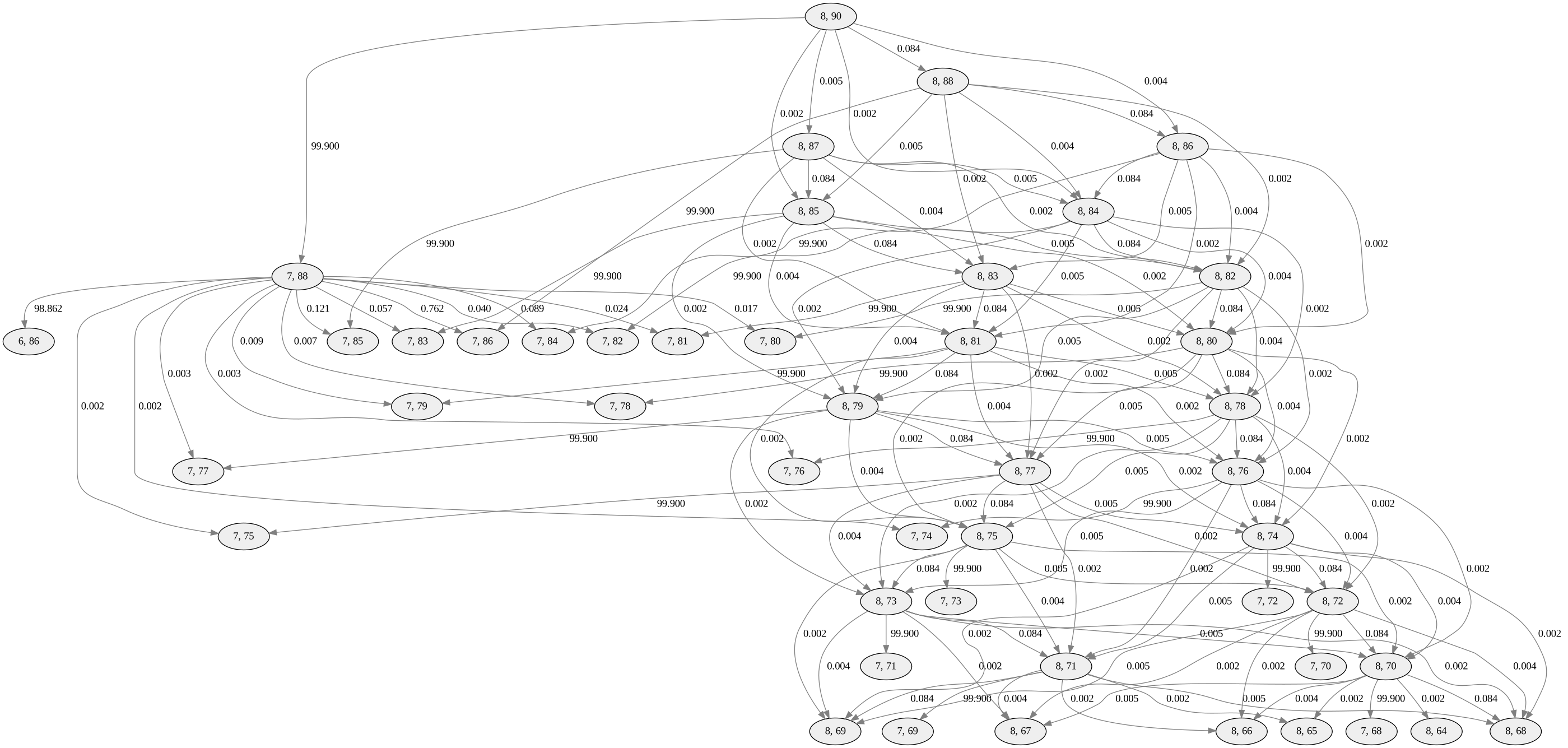
Since modeling the state of The Balance with all possible piles and decks will require a combinatorial explosion of vertices, we instead model states with a pair of numbers: the number of discrete values among the piles and the number of cards remaining among the hands and deck. The initial state is (8, 90). The winning state is (1, _) with any number of cards left. This is a model and thus “wrong,” but we suspect is “useful.” (Notably, this model does not include the choice of increasing the number of diverse values within the piles. Additionally, the probabilities assume the least number of discards will be made even though in play a player may want to keep certain cards.)
Below is a visualization of The Balance’s Markov chain, with the depth of the chain limited for clarity. The initial state, (8, 90), is at the top, with a large transition probability to (7, 88), and a small probability to (8, 88), and much smaller to other values that require a discard. Each of the child states further expands based on the possible reduction in pile diversity, keeping the pile values, and keeping the pile values while also discarding.
For transparency, we provide the weighted adjacency matrix file in Matrix Market format.
Solving the iterated Markov chain, we can derive the probabilities of arriving in certain game states after a number of turns. The figure below plots the probability of any end state, the probability of the win state, and the probability of the loss state on a given turn.
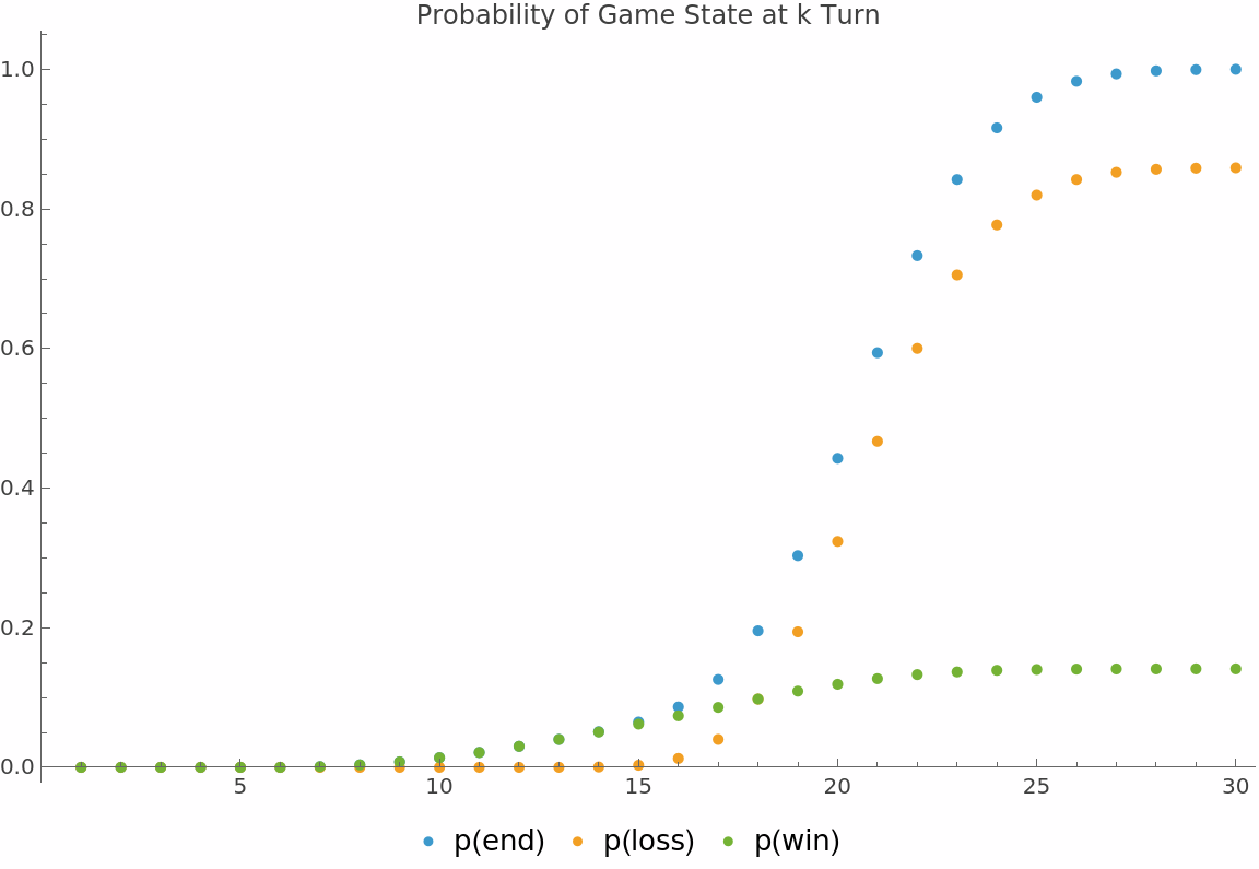
With this abstraction of the game rules, we find games end by the 30th turn as the normal consumption of cards plus forced discards consume the “run way.” Half of all games end in 20 or fewer turns. If the game ends early, it is more likely to be a win than a loss, but the probability of a loss quickly grows higher than a win by turn 19. Although longer games will almost inevitably end in defeat, median-length games have win rates in the range suggested by the poll.
Conclusion
The game designer’s choice of nine cards, eight piles, and a 90 card deck lead to a game where players have many “good” choices in the early and mid game, but a sharp transition to many difficult choices in the end game. Enlarging the deck would have little impact on the nature of choices and the end game would still be difficult, but there would be more turns to find a solution. However, with games probabilistically ending by turn 30 rather than the theoretical turn 45 maximum, the deck would need to be greatly increased in size for the number of expected turns to increase meaningfully.
Author Notes
I have no affiliation with New Venture Games. Analyzing abstract games is simply an enjoyable exercise.
As a possible item of confusion, the product page says The Balance has a “deck of 102 cards”. This is referencing the cards in the box, which contain 90 playable cards, 8 initial pile value card markers, and 4 player aid cards, not the playable deck size that we discuss above.
We used dot for the Markov chain visualization. We used Mathematica for computation of the Markov chain and creation of the probability plot.
References
(Wendl 2003) Wendl, Michael C. “Collision probability between sets of random variables.” Statistics & Probability Letters, Volume 64, Issue 3 (2003): Pages 249-254. doi
(Cassandras & Lafortune 2008) Cassandras, Christos G., and Stéphane Lafortune. 2008. Introduction to Discrete Event Systems. Boston: Kluwer Academic.